Chapter 11: Indexes

A customer calls Baldwin Bikes, the BikeStores shop in New York, about an order. The clerk types her surname into the support screen and waits. With 1,445 customers the answer comes back instantly. With 14 million, after a few years of growth and two acquisitions, the same screen takes forty seconds, and the nightly sales pipeline that joins orders to customers misses its window.

Nothing about the query changed. What changed is how much of the table SQL Server has to read to answer it, and that is what an index controls.

An index is the table's directory. It does not move a single customer; it tells SQL Server which page to open. This chapter opens up the storage engine to show what an index actually is, why it makes reads fast, and why every one you add makes writes a little slower. Every query runs against the BikeStores database, and every number in the output was measured on it.

Start by asking BikeStores which indexes it already has:

SELECT
    OBJECT_SCHEMA_NAME(i.object_id) + '.' + OBJECT_NAME(i.object_id) AS table_name,
    i.name      AS index_name,
    i.type_desc AS index_type
FROM sys.indexes AS i
INNER JOIN sys.tables AS t
    ON t.object_id = i.object_id
WHERE i.index_id > 0
ORDER BY table_name, i.index_id;

table_name            | index_name                     | index_type
----------------------+--------------------------------+-------------
production.brands     | PK__brands__5E5A8E27336842AE   | CLUSTERED
production.categories | PK__categori__D54EE9B434344679 | CLUSTERED
production.products   | PK__products__47027DF53F45974A | CLUSTERED
production.stocks     | PK__stocks__E68284D3DC40AC4D   | CLUSTERED
sales.customers       | PK__customer__CD65CB85FB6B74F6 | CLUSTERED
sales.order_items     | PK__order_it__837942D45CBDE54A | CLUSTERED
sales.orders          | PK__orders__46596229B2F7BEF4   | CLUSTERED
sales.staffs          | PK__staffs__1963DD9CBDECEBD9   | CLUSTERED
sales.staffs          | UQ__staffs__AB6E61644E0C4FA6   | NONCLUSTERED
sales.stores          | PK__stores__A2F2A30C597BDB3D   | CLUSTERED

Nobody wrote a CREATE INDEX for any of these. Every table got a clustered index the moment its PRIMARY KEY was declared in Chapter 9, and sales.staffs got a second one from its UNIQUE constraint on email. The suffixes are generated names, so yours will differ. By the end of this chapter you will know what each of those words means, and why the empty spaces in this list (no index on last_name, none on orders.customer_id) matter.

---

11.1 How SQL Server Stores a Row: The 8 KB Page

A query result looks like a spreadsheet, but SQL Server never stores one. On disk, a database is a set of data files cut into fixed-size blocks called pages, and every page is exactly 8 KB (8,192 bytes).

The page is the unit of all input and output. To read one customer, SQL Server reads the whole 8 KB page that holds her. That single fact explains most of what follows: query cost is counted in pages read, so a fast query is one that reads fewer pages.

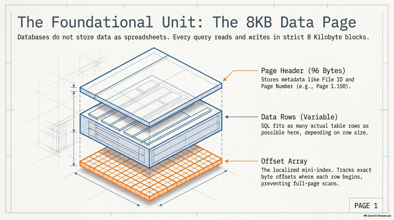
Every data page has three parts:

Part	Size	What it holds
Page header	Fixed 96 bytes	Metadata such as the file ID and page number, written as 1:150 (file 1, page 150)
Data rows	Variable	The table rows themselves, packed in until the page is full. Wider rows mean fewer rows per page
Offset array	2 bytes per row, at the end of the page	The byte position where each row starts, so SQL Server can jump to a row inside the page without reading from byte zero

You can see how BikeStores is laid out in pages:

SELECT
    OBJECT_SCHEMA_NAME(p.object_id) + '.' + OBJECT_NAME(p.object_id) AS table_name,
    SUM(p.rows)        AS row_count,
    SUM(a.data_pages)  AS data_pages
FROM sys.partitions AS p
INNER JOIN sys.allocation_units AS a
    ON a.container_id = p.partition_id
WHERE p.index_id IN (0, 1)
  AND OBJECT_SCHEMA_NAME(p.object_id) IN ('sales', 'production')
GROUP BY p.object_id
ORDER BY row_count DESC;

table_name            | row_count | data_pages
----------------------+-----------+-----------
sales.order_items     | 4722      | 23
sales.orders          | 1615      | 7
sales.customers       | 1445      | 19
production.stocks     | 939       | 3
production.products   | 321       | 3
sales.staffs          | 10        | 1
production.brands     | 9         | 1
production.categories | 7         | 1
sales.stores          | 3         | 1

All 1,445 customers fit in 19 pages, about 76 rows per page. sales.orders has more rows but fewer pages because its rows are narrower: a few integers and dates against the customer table's names, emails and addresses.

The offset array is a tiny index for a single page. What it cannot tell you is which of those 19 pages to open. That is the job of a real index, and the clearest way to see why you need one is to look at a table that does not have one.

---

11.2 Heaps and the Full Table Scan

A table with no clustered index is a heap. Rows go wherever there is free space, in whatever order they arrive. Think of a desk drawer you toss papers into: putting a paper in is instant, finding one later means going through the whole drawer.

Every BikeStores table has a clustered index, so make a heap to look at. SELECT ... INTO copies the rows but not the primary key or its index:

SELECT *
INTO sales.customers_heap
FROM sales.customers;

Now ask the heap for customer 14, with SET STATISTICS IO ON so SQL Server reports how many pages it read:

SET STATISTICS IO ON;

SELECT customer_id, first_name, last_name, city, state
FROM sales.customers_heap
WHERE customer_id = 14;

customer_id | first_name | last_name | city   | state
------------+------------+-----------+--------+------
14          | Garry      | Espinoza  | Forney | TX

Table 'customers_heap'. Scan count 1, logical reads 19

Logical reads is the number of 8 KB pages read (SQL Server prints a few more counters on that line; this book trims them). Nineteen pages is the whole table. SQL Server had no idea which page held Garry, so it did the only thing it could: a full table scan. It read page 1 and checked every row, then page 2, and kept going to the last page, because nothing told it there was not a second customer 14 further on. The execution plan names the operation Table Scan.

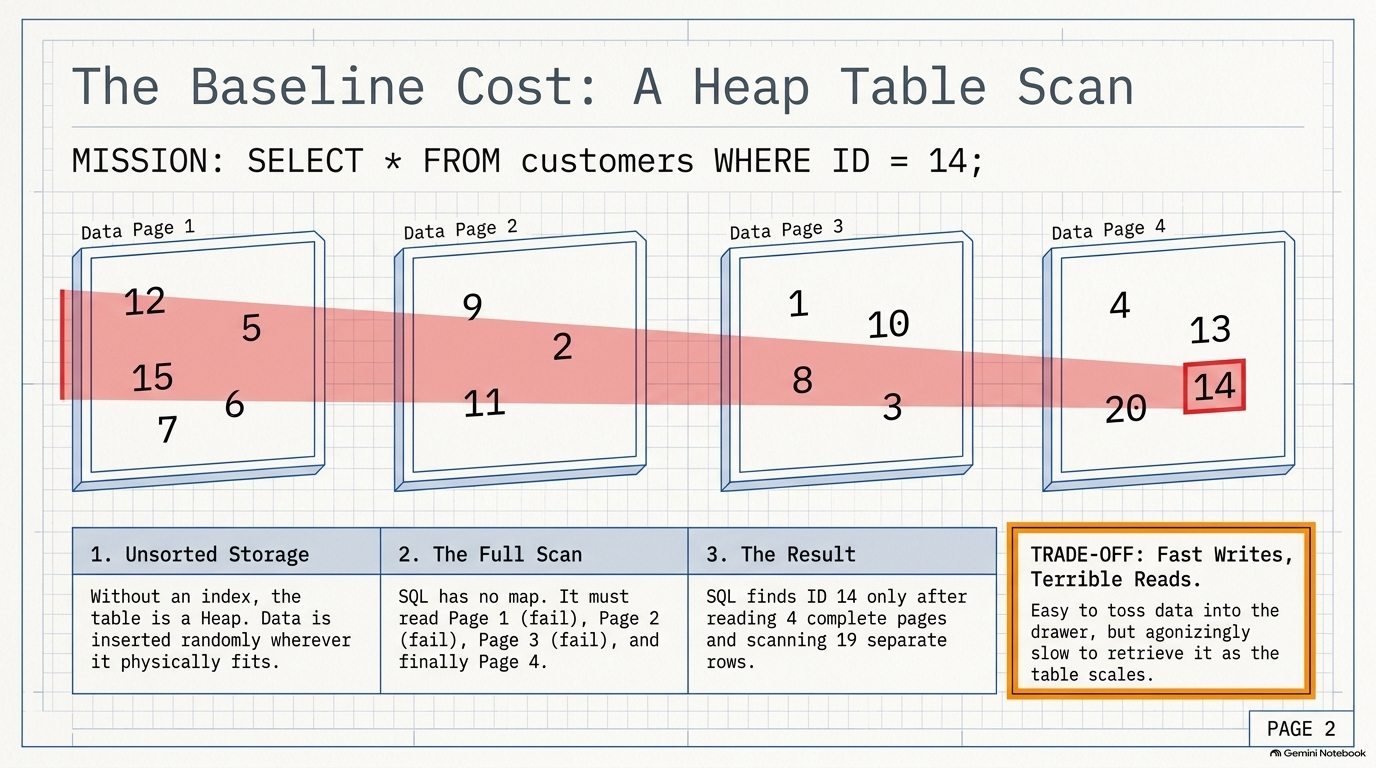
Scale it up and the cost scales with it. A customer table that fills 500,000 pages needs 500,000 page reads for every lookup, however few rows come back.

Heap	Behavior
Storage order	Whatever order rows were inserted
Insert speed	Fastest, since a row goes into the next free space
Lookup speed	Slowest, since every lookup scans every page
Good fit	Staging tables loaded in bulk and read once in full

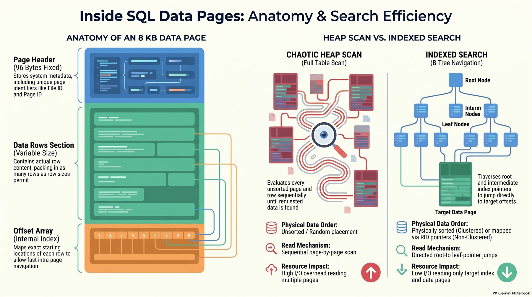
The scan is slow because the engine has no map. The right-hand side of this diagram is where the chapter is going: a structure that lets SQL Server walk straight to the page it needs.

---

11.3 The B-Tree: A Map of the Pages

The map SQL Server uses is a B-tree (balanced tree): a hierarchy of index pages in which each level splits the key range into smaller pieces, so every step down throws away most of the table.

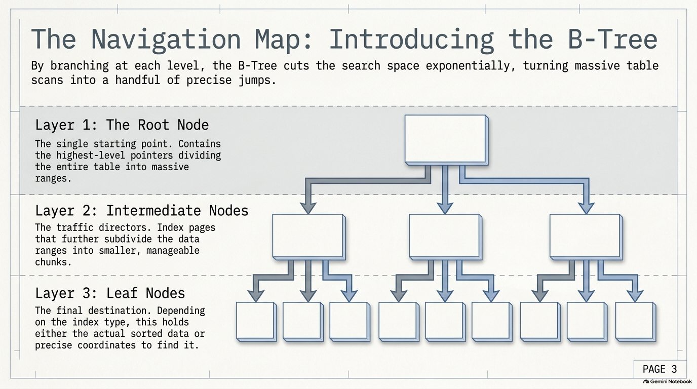
Level	Role
Root node	The single entry point. Holds key ranges that divide the whole table into a few large chunks
Intermediate nodes	Zero or more levels of index pages that split those ranges into smaller ones
Leaf nodes	The bottom level. Depending on the index type, they hold either the rows themselves or the address of each row

"Balanced" means every leaf is the same distance from the root, so any lookup costs the same number of page reads whichever key you ask for.

You can measure the real tree under sales.customers:

SELECT
    s.index_level,
    s.page_count,
    s.record_count
FROM sys.dm_db_index_physical_stats(
         DB_ID(), OBJECT_ID('sales.customers'), 1, NULL, 'DETAILED') AS s
ORDER BY s.index_level DESC;

index_level | page_count | record_count
------------+------------+-------------
1           | 1          | 19
0           | 19         | 1445

Level 1 is the root: one page holding 19 entries, one per leaf page. Level 0 is the leaf level: the 19 pages holding all 1,445 customers. The tree is two levels deep, so any customer is two page reads away.

The tree also stays shallow as the table grows. One index page holds hundreds of key ranges, so each level multiplies the reach of the one above it. When sales.customers outgrows what one root page can point to, SQL Server adds an intermediate level, and three or four levels cover tens of millions of rows.

The tree has the same shape for both kinds of index. They differ in what sits at the leaf level, and the clustered index is the place to start.

---

11.4 Clustered Indexes: Tracing a Lookup

A clustered index does two things to a table:

1. It physically sorts the rows by the index key, from lowest to highest, across the data pages.
2. It builds a B-tree over those sorted pages.

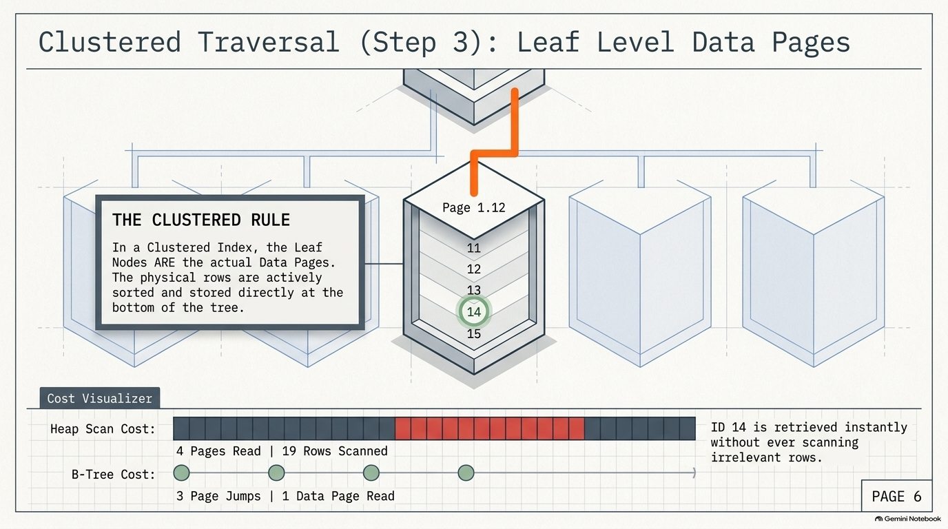
The defining rule is that the leaf level of a clustered index is the data itself. There is no separate copy of the rows. The table is the bottom of the tree.

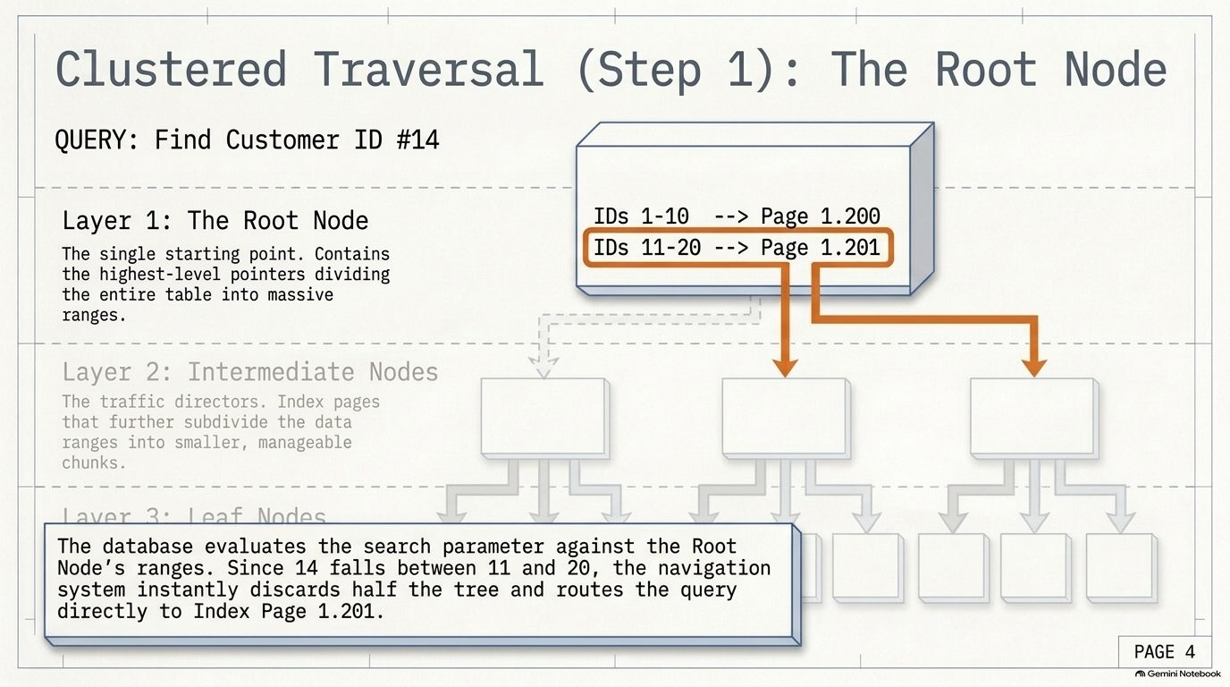
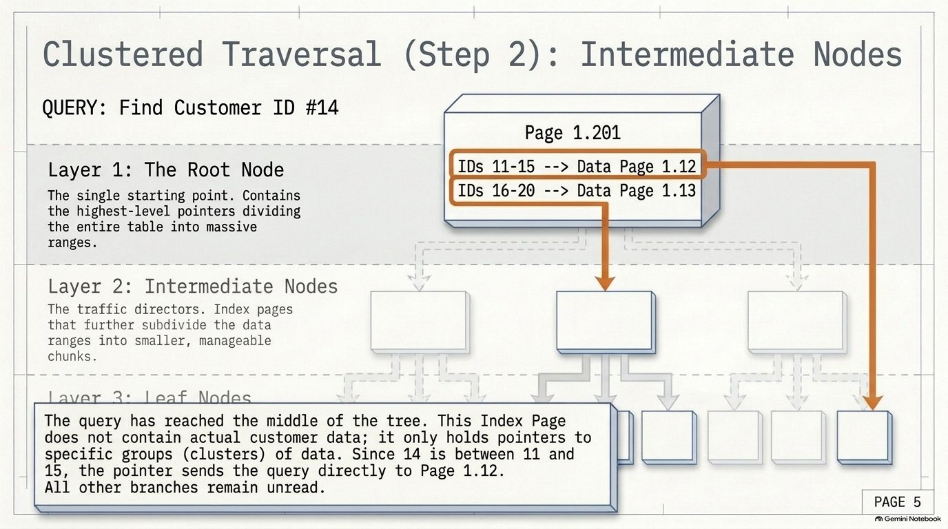
sales.customers is clustered on customer_id by its primary key. Here is the lookup for customer 14, step by step, as the diagrams draw it (with an intermediate level, as a bigger customer table would have).

Step 1, the root. The root page holds ranges: IDs 1-10 point one way, IDs 11-20 another. Since 14 falls in 11-20, everything else is discarded with one comparison.

Step 2, the intermediate node. That index page holds no customer data, only narrower ranges. IDs 11-15 point to one data page. Every other branch stays unread.

Step 3, the leaf. The leaf is an actual data page holding rows 11 to 15 in order. The offset array points straight at row 14, and the row is returned.

Now run the heap query from 11.2 against the real table:

SET STATISTICS IO ON;

SELECT customer_id, first_name, last_name, city, state
FROM sales.customers
WHERE customer_id = 14;

customer_id | first_name | last_name | city   | state
------------+------------+-----------+--------+------
14          | Garry      | Espinoza  | Forney | TX

Table 'customers'. Scan count 0, logical reads 2

Two pages: the root, then the one leaf page that holds Garry. The plan operator is Clustered Index Seek.

Because the rows are physically sorted, a clustered index is also very good at range queries. It seeks to the first key once, then reads forward through adjacent pages:

SELECT COUNT(*) AS customers
FROM sales.customers
WHERE customer_id BETWEEN 100 AND 200;

Query on 1,445 customers	Heap copy	Clustered on customer_id
customer_id = 14 (1 row)	19 reads, Table Scan	2 reads, Clustered Index Seek
customer_id BETWEEN 100 AND 200 (101 rows)	19 reads, Table Scan	4 reads, Clustered Index Seek

On 19 pages the gap is 19 against 2. On a 500,000-page table it is 500,000 against 3 or 4, because the scan grows with the table while the seek only grows with the depth of the tree.

There is one hard limit: a table can have only one clustered index, because rows can only be physically sorted one way. That is also why SQL Server builds one automatically when you declare a PRIMARY KEY, unless you write PRIMARY KEY NONCLUSTERED.

That leaves a question. Customers are sorted by customer_id, but the Baldwin Bikes clerk searches by surname. You cannot sort the table a second time, so you need a different kind of index.

---

11.5 Non-Clustered Indexes: A Separate Map

A non-clustered index leaves the table exactly as it is, heap or clustered, and builds a second B-tree beside it, sorted by its own key.

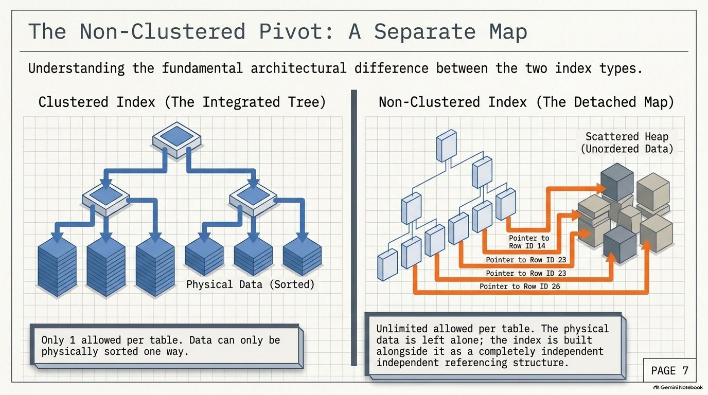
Its leaf level holds no rows. Each leaf entry holds the key value plus a row locator, the address of the full row. What that locator looks like depends on the table underneath:

Table underneath	Row locator stored in the leaf	Final step to fetch the row	Plan operator
Heap	A RID (row identifier): file, page and slot	Jump to that page and slot	RID Lookup
Clustered table	The clustered key value, e.g. customer_id = 758	Seek the clustered index with that key	Key Lookup

Watch it happen. Before any index on last_name, finding the one Garcia costs a full scan of the clustered index:

SET STATISTICS IO ON;

SELECT customer_id, first_name, last_name, email
FROM sales.customers
WHERE last_name = 'Garcia';

customer_id | first_name | last_name | email
------------+------------+-----------+------------------------
758         | Raymonde   | Garcia    | raymonde.garcia@aol.com

Table 'customers'. Scan count 1, logical reads 21

Add a non-clustered index on last_name and run it again:

CREATE INDEX ix_customers_last_name
ON sales.customers (last_name);

Table 'customers'. Scan count 1, logical reads 4

Twenty-one reads became four. The execution plan shows exactly where they went:

Nested Loops
  |--Index Seek     (ix_customers_last_name, last_name = 'Garcia')         2 reads
  |--Key Lookup     (PK__customer..., customer_id = 758)                    2 reads

The seek walks the new tree to the Garcia entry. That entry holds last_name and customer_id but not first_name or email, so SQL Server takes the customer_id and seeks the clustered index to fetch the rest of the row. That second step is the key lookup.

On the heap copy the same index ends in a RID instead, a physical address:

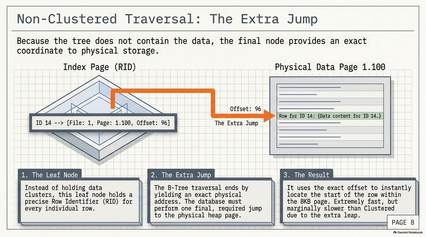
CREATE INDEX ix_customers_heap_last_name
ON sales.customers_heap (last_name);

SELECT customer_id, first_name, last_name, email
FROM sales.customers_heap
WHERE last_name = 'Garcia';

Table 'customers_heap'. Scan count 1, logical reads 3

Nested Loops
  |--Index Seek     (ix_customers_heap_last_name, last_name = 'Garcia')
  |--RID Lookup     (customers_heap)

That extra jump is the price of a non-clustered index, and it is paid once per matching row. Garcia matches one customer, so it is cheap. Larson matches seven, and seven lookups at two pages each cost more than reading the 19-page table straight through. Run the Larson query with the index in place and the optimizer ignores the index and scans the clustered index. Forcing the index anyway costs 16 reads.

That is not a bug. The optimizer estimates both plans and picks the cheaper one. A non-clustered index helps when it narrows the table to a small fraction of its rows; past that point, called the tipping point, a scan wins.

Unlike the clustered index, a table can have many non-clustered indexes (up to 999 in SQL Server). Each one is a separate structure that takes disk space and has to be maintained on every write.

---

11.6 Clustered vs Non-Clustered

The cleanest way to hold the two types in your head is to think of a printed book.

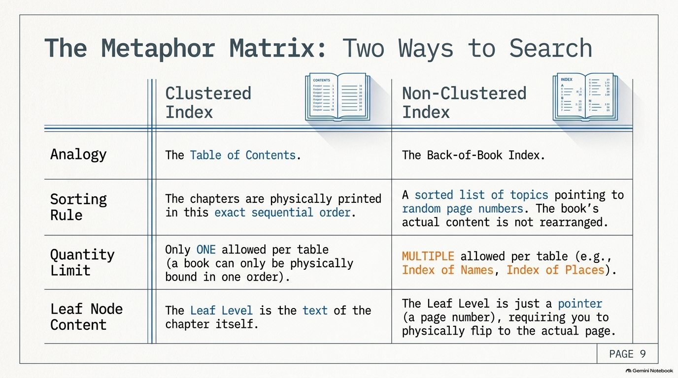
A clustered index is the book's page order. The chapters are physically bound in sequence, so there is only one ordering, and once you find your place you are reading the content itself.

A non-clustered index is the index at the back. It is a sorted list of topics with page numbers. A book can have several (an index of names, an index of places), and each entry sends you flipping to another page to read the actual text.

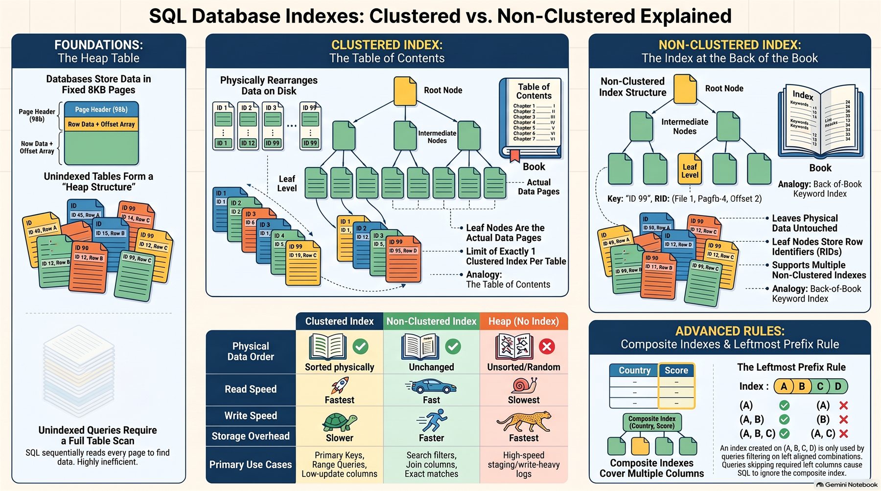
	Heap (no index)	Clustered index	Non-clustered index
Physical row order	Unsorted, insertion order	Sorted by the index key	Unchanged; the index is sorted, the table is not
Leaf level holds	(no tree)	The data rows themselves	Index key + row locator
Per table	n/a	One	Many
Single-row read	Slowest: full scan	Fastest: seek lands on the data	Fast: seek plus one lookup per row
Insert / update cost	Lowest	Moderate. Inserting into the middle of the order can force a page split	Each index adds one more tree to update on every write
Extra storage	None	Little, since the index is the table	A copy of the key columns for every row, per index
BikeStores example	sales.customers_heap	PK__customer__... on customer_id	ix_customers_last_name
Best candidates	Bulk-loaded staging tables	Primary keys, ever-increasing IDs, dates, range queries	Columns in frequent WHERE, JOIN and ORDER BY clauses

That "page split" cell is why the best clustered key is unique, narrow, ever-increasing and rarely updated, exactly like BikeStores' IDENTITY primary keys. A new customer always gets the next customer_id, so the row lands at the end of the last page and nothing in the middle is reshuffled. Clustering sales.customers on email instead would scatter inserts across the whole table, splitting pages in half to make room.

The whole comparison on one page:

---

11.7 Creating and Dropping Indexes

Index names follow a convention so they are easy to find in monitoring and in execution plans. This book uses ix_<table>_<columns>, lowercase like the rest of BikeStores.

The video walks through running index scripts like the ones below. Pause it and type each step yourself.

Non-clustered index

-- NONCLUSTERED is the default, so these two are identical
CREATE NONCLUSTERED INDEX ix_customers_last_name
ON sales.customers (last_name);

CREATE INDEX ix_customers_last_name
ON sales.customers (last_name);

Clustered index

sales.customers already has its clustered index, so ask for a second one and SQL Server refuses:

CREATE CLUSTERED INDEX ix_customers_email
ON sales.customers (email);

Msg 1902: Cannot create more than one clustered index on table 'sales.customers'.
Drop the existing clustered index 'PK__customer__CD65CB85FB6B74F6' before creating another.

The heap copy has none, so it accepts one:

CREATE CLUSTERED INDEX ix_customers_heap_customer_id
ON sales.customers_heap (customer_id);

Running this physically re-sorts the whole table. On a large production table that is a heavy, blocking operation to schedule, not to run casually.

Unique index

CREATE UNIQUE INDEX ix_customers_email
ON sales.customers (email);

A unique index speeds up lookups and also enforces a rule. All 1,445 BikeStores emails are distinct, so the index builds, and from then on a duplicate is rejected:

INSERT INTO sales.customers (first_name, last_name, email)
VALUES ('Test', 'Duplicate', 'garry.espinoza@hotmail.com');

Msg 2601: Cannot insert duplicate key row in object 'sales.customers' with unique index
'ix_customers_email'. The duplicate key value is (garry.espinoza@hotmail.com).
The statement has been terminated.

A UNIQUE constraint creates exactly this kind of index behind the scenes. That is where the UQ__staffs__... index on sales.staffs in the opening listing came from.

Dropping an index

DROP INDEX ix_customers_last_name ON sales.customers;

-- SQL Server 2016+: no error if it is already gone
DROP INDEX IF EXISTS ix_customers_last_name ON sales.customers;

An index that enforces a constraint cannot be dropped this way:

DROP INDEX PK__customer__CD65CB85FB6B74F6 ON sales.customers;

Msg 3723: An explicit DROP INDEX is not allowed on index
'sales.customers.PK__customer__CD65CB85FB6B74F6'.
It is being used for PRIMARY KEY constraint enforcement.

To remove it you drop the constraint with ALTER TABLE ... DROP CONSTRAINT, as in Chapter 9, which turns the table back into a heap. On sales.customers that would also fail while sales.orders has a foreign key pointing at it, which is the database protecting itself.

So far every index has had one column. Real queries usually filter on more than one, which brings in the rule people most often get wrong.

---

11.8 Composite Indexes and the Leftmost Prefix Rule

A composite index has more than one key column. It is sorted by the first column, then by the second within each value of the first, exactly like a phone book sorted by surname and then first name.

CREATE INDEX ix_customers_name
ON sales.customers (last_name, first_name);

Each column can carry its own sort direction, (last_name ASC, first_name DESC), which matters when a query's ORDER BY mixes directions.

The sort order produces the leftmost prefix rule: SQL Server can seek into a composite index only when the query filters on the leading column, then optionally the next one, without skipping any.

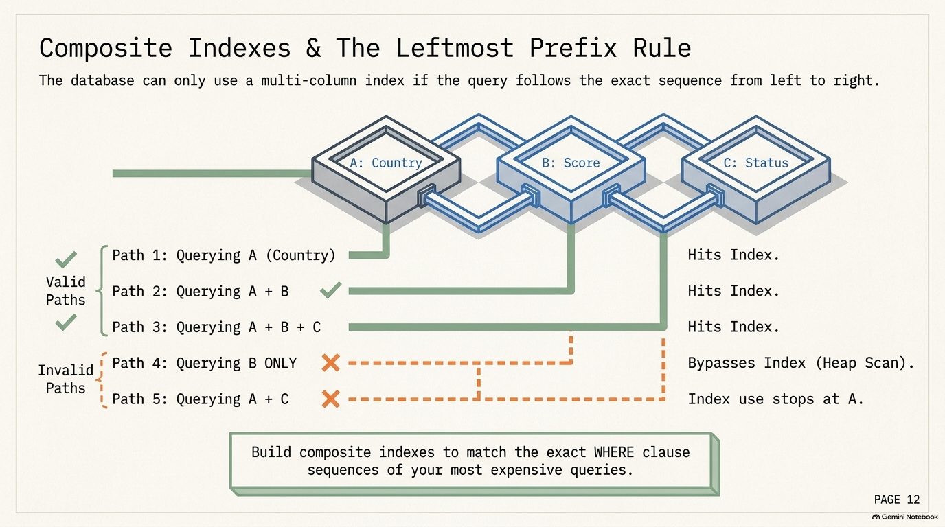
Three queries against ix_customers_name:

SET STATISTICS IO ON;

-- 1. Leading column only
SELECT customer_id, first_name, last_name
FROM sales.customers
WHERE last_name = 'Larson';

-- 2. Both columns
SELECT customer_id, first_name, last_name
FROM sales.customers
WHERE last_name = 'Joyner' AND first_name = 'Lizzie';

-- 3. Second column only
SELECT customer_id, first_name, last_name
FROM sales.customers
WHERE first_name = 'Lizzie';

Query	Plan	Logical reads
1. last_name = 'Larson' (7 rows)	Index Seek on ix_customers_name	2
2. last_name and first_name (1 row)	Index Seek on both key columns	2
3. first_name = 'Lizzie' (1 row)	Index Scan: every page of the index, checking each row	8

Query 3 finds the same single customer as query 2 and costs four times as much. Lizzies are spread across every surname in the index, so there is no starting point to seek to; the best SQL Server can do is read the whole index. (Query 1 needs no key lookup even for seven rows, because customer_id, the clustered key, rides along in every non-clustered index and both name columns are in the key.)

For an index on (A, B, C):

Query filters on	Can the index seek?	Why
A	Yes	Leading column
A and B	Yes	Unbroken prefix
A, B and C	Yes	Full key
B only	No	Values of B are scattered across every A. Best case, an index scan
A and C	Partly	Seeks on A, then checks C row by row, because B is skipped

So build composite indexes to match the WHERE clauses of your most expensive queries, and put the column you always filter on first. When two columns are always filtered together, lead with the more selective one (more distinct values; BikeStores has 753 surnames but only 3 states) unless another query also needs the other column on its own.

---

11.9 Covering Indexes with INCLUDE

Section 11.5 showed that every row a non-clustered index finds costs one extra lookup. You can remove that lookup entirely when the index already contains every column the query needs. Such an index covers the query.

Mount Vernon, NY is BikeStores' biggest city, with 20 customers. Marketing wants their names and emails:

SELECT first_name, last_name, email
FROM sales.customers
WHERE city = 'Mount Vernon';

With a plain index on city, the optimizer weighs 20 key lookups against reading the table and chooses the table:

CREATE INDEX ix_customers_city ON sales.customers (city);

Table 'customers'. Scan count 1, logical reads 21     -- Clustered Index Scan, index ignored

Force the index with a hint, WITH (INDEX(ix_customers_city)), and it costs 42 reads, twice as much, because each of the 20 rows needs its own lookup. The optimizer was right. Now replace the index with one that carries the columns the query returns:

DROP INDEX ix_customers_city ON sales.customers;

CREATE INDEX ix_customers_city_cover
ON sales.customers (city)
INCLUDE (first_name, last_name, email);

Table 'customers'. Scan count 1, logical reads 4      -- Index Seek, no lookups

INCLUDE columns are stored only at the leaf level. They are not part of the sort key, so they cost less than adding them to the key and do not affect the leftmost prefix rule. The query is now answered from the index alone and never touches the table.

Index on city	Plan	Logical reads
Plain, optimizer's choice	Clustered Index Scan	21
Plain, forced with a hint	Index Seek + 20 Key Lookups	42
Covering with INCLUDE	Index Seek	4

Put a column in...	When
The key ( ... )	You filter, join or sort on it
INCLUDE ( ... )	You only return it in the SELECT list

The numbers in this chapter all came from two tools, and you will use them every time you tune a query.

---

11.10 Seeing the Difference: STATISTICS IO and Execution Plans

SET STATISTICS IO ON reports how many pages each statement read. Logical reads is the number to watch: it does not change with caching or server load, so it is the fairest before-and-after comparison.

The execution plan (Ctrl+M in SSMS turns on the actual plan) names the operation SQL Server chose. Every operator in this chapter appeared in a real BikeStores plan:

Plan operator	Meaning	Seen in this chapter
Table Scan	Read every page of a heap	customers_heap, customer 14
Clustered Index Scan	Read every page of a clustered table	last_name = 'Garcia' before indexing
Clustered Index Seek	Navigate the clustered tree straight to the rows	customer_id = 14
Index Seek	Navigate a non-clustered tree	ix_customers_last_name, ix_customers_city_cover
Index Scan	Read every page of a non-clustered index	first_name = 'Lizzie'
Key Lookup / RID Lookup	The extra jump from a non-clustered leaf to the row	Garcia, on the clustered table and on the heap
Sort	Order rows that did not arrive in order	Section 11.12, before the index

A seek navigates the tree; a scan reads everything. Most index tuning comes down to turning the scans that matter into seeks, and removing lookups and sorts.

To see what indexes a table has now, query the catalog. After the indexes from sections 11.7 to 11.9 are in place on sales.customers:

SELECT
    i.name        AS index_name,
    i.type_desc   AS index_type,
    i.is_unique,
    c.name        AS column_name,
    ic.key_ordinal,
    ic.is_included_column
FROM sys.indexes AS i
INNER JOIN sys.index_columns AS ic
    ON i.object_id = ic.object_id
   AND i.index_id  = ic.index_id
INNER JOIN sys.columns AS c
    ON ic.object_id = c.object_id
   AND ic.column_id = c.column_id
WHERE i.object_id = OBJECT_ID('sales.customers')
ORDER BY i.index_id, ic.is_included_column, ic.key_ordinal;

index_name                     | index_type   | is_unique | column_name | key_ordinal | is_included_column
-------------------------------+--------------+-----------+-------------+-------------+-------------------
PK__customer__CD65CB85FB6B74F6 | CLUSTERED    | 1         | customer_id | 1           | 0
ix_customers_name              | NONCLUSTERED | 0         | last_name   | 1           | 0
ix_customers_name              | NONCLUSTERED | 0         | first_name  | 2           | 0
ix_customers_city_cover        | NONCLUSTERED | 0         | city        | 1           | 0
ix_customers_city_cover        | NONCLUSTERED | 0         | first_name  | 0           | 1
ix_customers_city_cover        | NONCLUSTERED | 0         | last_name   | 0           | 1
ix_customers_city_cover        | NONCLUSTERED | 0         | email       | 0           | 1
ix_customers_email             | NONCLUSTERED | 1         | email       | 1           | 0

Included columns show key_ordinal = 0 because they are not part of the sort. Those indexes are not free, which is what the next section is about.

---

11.11 The Cost of an Index: When Not to Index

If indexes make reads fast, why not index every column? Because every index is a second copy of some data that must be kept in sync, and it takes space.

SELECT i.name AS index_name, SUM(a.used_pages) AS used_pages
FROM sys.indexes AS i
INNER JOIN sys.partitions AS p
    ON p.object_id = i.object_id AND p.index_id = i.index_id
INNER JOIN sys.allocation_units AS a
    ON a.container_id = p.partition_id
WHERE i.object_id = OBJECT_ID('sales.customers')
GROUP BY i.name, i.index_id
ORDER BY i.index_id;

index_name                     | used_pages
-------------------------------+-----------
PK__customer__CD65CB85FB6B74F6 | 21
ix_customers_name              | 9
ix_customers_city_cover        | 15
ix_customers_email             | 9

The table itself is 21 pages. The three indexes added in this chapter come to 33 more, so the customer data now takes more than twice its own size. Every INSERT into sales.customers now writes four structures instead of one, every UPDATE to a name, city or email moves entries in the affected indexes, and every DELETE removes an entry from each.

Some indexes do not even pay for themselves on reads. An index on state looks useful until you check the data: 1,019 of the 1,445 customers are in NY. Even state = 'TX', 142 customers, is past the tipping point. In both cases the optimizer ignores the index and scans the table, so you pay to maintain it and never use it.

Situation	Index?	Reason
Column in frequent WHERE, JOIN or ORDER BY on a large table	Yes	Turns scans into seeks
Foreign key column, e.g. sales.orders.customer_id	Usually	Joins and cascading checks scan without one
Small table, a few pages	Rarely	Scanning three pages is already as cheap as seeking
Low-selectivity column, e.g. sales.customers.state	Rarely	Returns a large share of the table, so the optimizer scans anyway
Write-heavy table, e.g. event logs, staging loads	Sparingly	Each index slows every insert
Column that is rarely queried	No	Pure write and storage cost with nothing in return

The foreign key row deserves a closer look, because BikeStores has none indexed. Looking up Garry Espinoza's orders:

SELECT order_id, order_date, order_status, store_id
FROM sales.orders
WHERE customer_id = 14;

order_id | order_date | order_status | store_id
---------+------------+--------------+---------
357      | 2016-08-05 | 3            | 3
419      | 2016-09-04 | 4            | 3
1572     | 2018-04-22 | 1            | 3

Table 'orders'. Scan count 1, logical reads 9     -- whole table

With CREATE INDEX ix_orders_customer_id ON sales.orders (customer_id); it drops to 8 reads (an index seek plus three key lookups). At 7 data pages, sales.orders is too small for the index to matter much, and that is an honest result. But the scan grows with every order the shops take, while the seek stays at a handful of pages. That is why foreign keys are indexed by default in most production schemas, even when the difference is invisible on day one.

An index is a trade, not a free upgrade. No indexes gives you the fastest writes and the slowest reads; too many gives you the reverse. The job is to index for the queries you actually run, and to drop the ones nobody uses.

For data engineers this matters most in pipelines. A common bulk-load pattern is to drop or disable non-clustered indexes on the target table, load the batch into a bare structure, then rebuild the indexes once, instead of maintaining them row by row through millions of inserts.

---

11.12 Putting It Together

Baldwin Bikes (store_id = 2) runs a quarterly report of its orders, sorted by date, many times a day during quarter close:

SET STATISTICS IO ON;

SELECT order_id, customer_id, order_date, order_status
FROM sales.orders
WHERE store_id = 2
  AND order_date BETWEEN '2018-01-01' AND '2018-03-31'
ORDER BY order_date;

It returns 108 orders. Without an index the plan is a Clustered Index Scan of all of sales.orders (9 logical reads) feeding a Sort, because the rows come out in order_id order and the report wants order_date.

The fix is one index designed from the query:

CREATE INDEX ix_orders_store_date
ON sales.orders (store_id, order_date)
INCLUDE (customer_id, order_status);

order_id | customer_id | order_date | order_status
---------+-------------+------------+-------------
1324     | 862         | 2018-01-01 | 4
1327     | 1026        | 2018-01-02 | 4
1328     | 1083        | 2018-01-02 | 4
1330     | 761         | 2018-01-04 | 4
1331     | 1122        | 2018-01-05 | 4
...
(108 rows)

Table 'orders'. Scan count 1, logical reads 2

The plan is now a single Index Seek, with no lookup and no sort. Why each choice holds up:

Choice	Reason
store_id leads the key	It is the equality filter, so the seek jumps straight to store 2's block
order_date second	Within store 2, dates are sorted, so the BETWEEN becomes a range seek and the rows come out already in ORDER BY order. No Sort operator
customer_id, order_status in INCLUDE	Returned but not filtered on: covered, so no key lookup per row
order_id not listed	It is the clustered key, so every non-clustered index already carries it

	Before	After
Plan	Clustered Index Scan + Sort	Index Seek
Logical reads	9	2
Grows with	Every order in every store	Only store 2's orders in the date range

That last row is the real payoff. Today the difference is seven pages. When the three shops have ten years of orders, the scan reads all of them and the seek still reads one quarter of one store.

If you followed along in your own BikeStores, put it back the way it was so later chapters see the same database:

DROP INDEX IF EXISTS ix_customers_last_name ON sales.customers;
DROP INDEX IF EXISTS ix_customers_name ON sales.customers;
DROP INDEX IF EXISTS ix_customers_city ON sales.customers;
DROP INDEX IF EXISTS ix_customers_city_cover ON sales.customers;
DROP INDEX IF EXISTS ix_customers_email ON sales.customers;
DROP INDEX IF EXISTS ix_orders_customer_id ON sales.orders;
DROP INDEX IF EXISTS ix_orders_store_date ON sales.orders;
DROP TABLE IF EXISTS sales.customers_heap;

---

Summary

SQL Server stores every table in 8 KB pages, and query cost is measured in pages read: all 1,445 BikeStores customers fit in 19. A table with no clustered index is a heap: rows sit in insertion order, inserts are cheap, and every lookup is a full table scan.

An index is a B-tree of index pages that narrows the search level by level, from the root through any intermediate nodes to the leaves. In a clustered index the leaves are the data pages and the rows are physically sorted, so there can be only one per table; every BikeStores table got one from its PRIMARY KEY. In a non-clustered index the leaves hold the key plus a row locator (a RID on a heap, the clustered key otherwise), so fetching the rest of the row costs a lookup, and a table can have many.

Composite indexes follow the leftmost prefix rule: they can only seek on an unbroken run of leading columns. INCLUDE adds non-key columns so an index can cover a query and skip the lookups. SET STATISTICS IO and the execution plan show whether a query seeks or scans. Every index speeds up some reads and slows every write, so index for the queries you actually run.

---

Check Your Understanding

Flashcards

Read the question, answer it in your head, then open the card.

1. 01 / 10What is the fixed size of a standard data page in a SQL database?Reveal answer

   8 KB.
2. 02 / 10In a SQL database data page, what information is stored in the 96-byte page header?Reveal answer

   Metadata about the page, such as the Page ID (composed of File ID and Page Number).
3. 03 / 10What is the purpose of the offset array located at the end of a database data page?Reveal answer

   It tracks where each row begins inside the page, enabling SQL to locate specific rows without scanning the entire page byte by byte.
4. 04 / 10What performance tradeoff characterizes a Heap table?Reveal answer

   Very fast write (INSERT) operations, but very slow read (SELECT) operations.
5. 05 / 10What operation occurs when SQL scans an unindexed table page by page and row by row to satisfy a query?Reveal answer

   A full table scan.
6. 06 / 10What physical change occurs to table data when a clustered index is created?Reveal answer

   SQL physically sorts and rearranges all data rows within the data pages based on the indexed key column.
7. 07 / 10How does creating a non-clustered index alter the physical arrangement of existing data pages?Reveal answer

   It does not alter the physical arrangement at all; data pages remain completely untouched.
8. 08 / 10Why are primary keys considered ideal candidates for a clustered index?Reveal answer

   Primary key values are unique and rarely updated, preventing costly physical page re-sorting during updates.
9. 09 / 10In SQL Server, what index type is automatically created by default when a Primary Key constraint is defined?Reveal answer

   A Clustered Index.
10. 10 / 10Why does a non-clustered index require more overall database storage space than a clustered index?Reveal answer

    It allocates a dedicated, separate B-tree structure with its own set of index pages and pointers.

Quiz

Thirteen questions on the whole chapter. Pick an answer to see why each option is right or wrong; questions marked Select all that apply need every correct option ticked before you check.

1. 01In a relational database system like SQL Server, what is the fixed storage size of a data page, and what information is stored within its header section?
2. 02What process does the database engine use when searching for a specific record in a table that lacks a clustered index (a heap structure)?
3. 03In the B-tree structure of a clustered index, what resides specifically at the leaf level?
4. 04Select all that applyWhich of the following statements accurately describe the structure and mechanics of a non-clustered index?
5. 05Why can a relational database table have only one clustered index?
6. 06How do clustered indexes compare to non-clustered indexes with respect to write performance (INSERT operations)?
7. 07When a non-clustered index is created on a heap table, what three components compose the Row Identifier (RID) stored in the index page?
8. 08Select all that applyWhich of the following characteristics make a column an ideal candidate for a clustered index?
9. 09Examine the following T-SQL command: CREATE INDEX ix_customers_last_name ON sales.customers (last_name); Which type of index will be created by default?
10. 10What index creation behavior occurs automatically in SQL Server when a PRIMARY KEY constraint is defined on a new table?
11. 11A composite non-clustered index is defined as CREATE INDEX ix_customers_state_city ON sales.customers (state, city); Which of the following queries CANNOT seek on this composite index?
12. 12Suppose a composite index is defined on four columns in the following order: (A, B, C, D). Which query filtering combination will fail to use the index due to the leftmost prefix rule?
13. 13Select all that applyWhy does adding multiple non-clustered indexes to a table increase storage consumption compared to having only a clustered index?

0 / 13 correct0 of 13 answered

---

Exercises

11.1 - Create sales.orders_heap as a heap copy of sales.orders using SELECT ... INTO. Run SELECT * FROM sales.orders_heap WHERE order_id = 1200; with SET STATISTICS IO ON and record the logical reads. Run the same query against sales.orders and explain the difference using the plan operators.

11.2 - sales.order_items has no index on product_id. Write a query that returns every order line for product_id = 7, record its logical reads and plan, then create an index that turns it into a seek. Is there a Key Lookup? Change the index so there is not.

11.3 - Write a query against sys.indexes and sys.index_columns that lists every index in the production schema with its key and included columns.

11.4 - An index exists on production.products (brand_id, model_year). For each query, say whether it can seek on the index and why:

-- a
SELECT product_name FROM production.products WHERE brand_id = 9;
-- b
SELECT product_name FROM production.products WHERE model_year = 2018;
-- c
SELECT product_name FROM production.products WHERE brand_id = 9 AND model_year = 2018;

11.5 - The following statement fails. Explain why, and write the two different ways you could make email the clustered key of sales.customers (and what each would cost):

CREATE CLUSTERED INDEX ix_customers_email
ON sales.customers (email);
-- Msg 1902: Cannot create more than one clustered index on table 'sales.customers'.

11.6 - Design the indexes for production.products to support both of these frequent queries. Justify the column order and any INCLUDE list:

SELECT product_name, list_price FROM production.products WHERE brand_id = @b ORDER BY list_price;
SELECT product_name FROM production.products WHERE category_id = @c AND model_year = @y;

11.7 - Think About It: BikeStores grows to 30 million order lines, loaded nightly into sales.order_items, which now has six non-clustered indexes, and the load takes four hours. A teammate proposes dropping all six indexes permanently. Another proposes leaving them. What would you do instead, and what would you measure before and after to prove it worked?